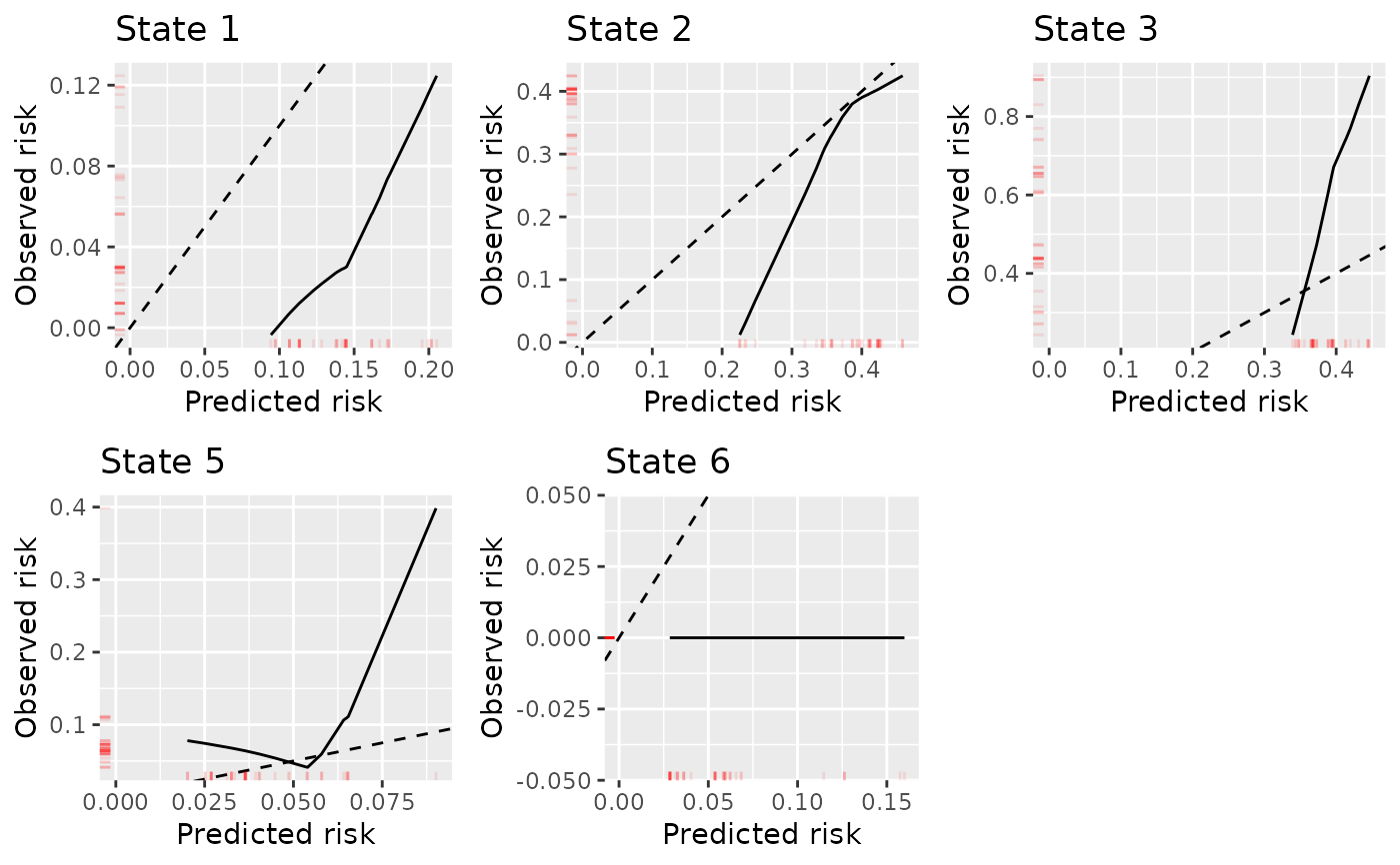
Plots calibration curves for the transition probabilities of a multistate model
estimated using calib_pv.
Usage
# S3 method for calib_pv
plot(x, ..., combine = TRUE, ncol = NULL, nrow = NULL, transparency.rug = 0.1)
Arguments
- x
Object of class 'calib_pseudo' generated from
calib_pv.- ...
Other
- combine
Whether to combine into one plot using ggarrange, or return as a list of individual plots
- ncol
Number of columns for combined calibration plot
- nrow
Number of rows for combined calibration plot
- transparency.rug
Degree of transparency for the density rug plot along each axis
Value
If combine = TRUE, returns an object of classes gg, ggplot, and ggarrange,
as all ggplots have been combined into one object. If combine = FALSE, returns an object of
class list, each element containing an object of class gg and ggplot.
Examples
# Using competing risks data out of initial state (see vignette: ... -in-competing-risk-setting).
# Estimate and plot pseudo-value calibration curves for the predicted transition
# probabilities at time t = 1826, when predictions were made at time
# s = 0 in state j = 1. These predicted transition probabilities are stored in tp.cmprsk.j0.

# To minimise example time we reduce the datasets to 50 individuals.
# Extract the predicted transition probabilities out of state j = 1 for first 50 individuals
tp.pred <- tp.cmprsk.j0 |>
 dplyr::filter(id %in% 1:50) |>
 dplyr::select(any_of(paste("pstate", 1:6, sep = "")))
# Reduce ebmtcal to first 50 individuals
ebmtcal <- ebmtcal |> dplyr::filter(id %in% 1:50)
# Reduce msebmtcal.cmprsk to first 50 individuals
msebmtcal.cmprsk <- msebmtcal.cmprsk |> dplyr::filter(id %in% 1:50)

# Now estimate the observed event probabilities for each possible transition.
dat.calib.pv <- calib_pv(data.mstate = msebmtcal.cmprsk,
  data.raw = ebmtcal,
  j = 1,
  s = 0,
  t = 1826,
  tp.pred = tp.pred,
  curve.type = "loess",
  loess.span = 1,
  loess.degree = 1)

 # These are then plotted
 plot(dat.calib.pv, combine = TRUE, nrow = 2, ncol = 3)