Comparison-in-competing-risks-setting
Source:vignettes/articles/Comparison-in-competing-risks-setting.Rmd
Comparison-in-competing-risks-setting.RmdData preperation
This vignette compares the calibration of a competing risks model
assessed using the approaches provided in calibmsm,
namely the BLR-IPCW and pseudo-value approaches, with graphical
calibration curves developed by Austin et al.
(2022). We use data from the European Society for Blood and
Marrow Transplantation (EBMT 2023), which
contains multistate survival data after a transplant for patients with
blood cancer. The start of follow up is the day of the transplant and
the initial state is alive and in remission. There are three
intermediate events
(:
recovery,
:
adverse event, or
:
recovery + adverse event), and two absorbing states
(:
relapse and
:
death). This data was originally made available from the
mstate package (Wreede, Fiocco, and
Putter 2011). For this example, we treat the transitions out of
the first state as a standalone competing risks model by setting all
subsequent states to be absorbing states. We are ignoring the subsequent
multistate aspect of the data.
We first load the predicted transition probabilities for each
individual from this model, which are provided in the dataset
tp_cmprsk_j0. The code for deriving this is available in
the source code for the package (see
prepare_vignette_cmprsk_data.R). These are generated by
specifying the transition matrix to define the competing risks model
(i.e. all subsequent states to act as absorbing states), and then
generate predicted risks (cumulative incidence functions) using the
theory of Putter, Fiocco, and Geskus
(2007). These are derived using the software in
mstate (Wreede, Fiocco, and Putter
2011). Predicted risks were generated for each individual using a
leave-one-out approach (i.e. each individual was removed from the
dataset before fitting the competing risks model and estimating a
predicted risk for that individual). The following four variables were
used to estimate the predicted risks: year of transplant
(year), age at transplant (age), prophylaxis
given (proph), and whether the donor was gender matched
(match).
The transition probabilities are stored in the object
tp_cmprsk_j0. Datasets in formats required for function
calib_msm are stored in ebmtcal.cmprsk
(data_raw argument) and msebmtcal_cmprsk
(data_ms argument). Note that the
ebmtcal.cmprsk is the same ebmtcal except the
variables dtcens and dtcens.s have been
derived in a different manner. Specifically, in this setting entry into
any state will have the effect of preventing censoring as they are all
absorbing states, whereas in ebmtcal this was true only for
entry into states 5 and 6, however this is the
only difference between the two datasets, A completely new dataset for
the data.ms argument was required, which reflects the fact
this is now a competing risks data structure. Please refer to the Overview
vignette for more details about how these datasets should be
formatted, and refer to the source code for specifically how these two
datasets were derived. We assess calibration at 5 years (1826 days) for
all methods.
library(calibmsm)

data("tp_cmprsk_j0")
head(tp_cmprsk_j0)
#>   id   pstate1   pstate2   pstate3 pstate4    pstate5    pstate6        se1
#> 1  1 0.1135057 0.4093590 0.3964498       0 0.02688596 0.05379955 0.01291270
#> 2  2 0.1135518 0.4114981 0.3942408       0 0.02689840 0.05381085 0.01291690
#> 3  3 0.1131989 0.4117482 0.3944988       0 0.02681945 0.05373457 0.01289565
#> 4  4 0.1376981 0.3870386 0.3728509       0 0.04027730 0.06213511 0.01858789
#> 5  5 0.1227877 0.4277392 0.3496972       0 0.03130458 0.06847131 0.01945048
#> 6  6 0.1131989 0.4117482 0.3944988       0 0.02681945 0.05373457 0.01289565
#>          se2        se3 se4         se5         se6
#> 1 0.01918215 0.01874680   0 0.006339773 0.007719292
#> 2 0.01920148 0.01870398   0 0.006342388 0.007719937
#> 3 0.01921355 0.01871733   0 0.006325238 0.007708340
#> 4 0.02447306 0.02323096   0 0.010698591 0.010818696
#> 5 0.02777129 0.02476595   0 0.009947925 0.012554747
#> 6 0.01921355 0.01871733   0 0.006325238 0.007708340

data("ebmtcal_cmprsk")
head(ebmtcal_cmprsk)
#>   id  rec rec.s   ae ae.s recae recae.s  rel rel.s  srv srv.s      year agecl
#> 1  1   22     1  995    0   995       0  995     0  995     0 1995-1998 20-40
#> 2  2   29     1   12    1    29       1  422     1  579     1 1995-1998 20-40
#> 3  3 1264     0   27    1  1264       0 1264     0 1264     0 1995-1998 20-40
#> 4  4   50     1   42    1    50       1   84     1  117     1 1995-1998 20-40
#> 5  5   22     1 1133    0  1133       0  114     1 1133     0 1995-1998   >40
#> 6  6   33     1   27    1    33       1 1427     0 1427     0 1995-1998 20-40
#>   proph              match dtcens dtcens_s
#> 1    no no gender mismatch     22        0
#> 2    no no gender mismatch     12        0
#> 3    no no gender mismatch     27        0
#> 4    no    gender mismatch     42        0
#> 5    no    gender mismatch     22        0
#> 6    no no gender mismatch     27        0

data("msebmtcal_cmprsk")
head(msebmtcal_cmprsk)
#>   id from to trans Tstart Tstop time status
#> 1  1    1  2     1      0    22   22      1
#> 2  1    1  3     2      0    22   22      0
#> 3  1    1  5     3      0    22   22      0
#> 4  1    1  6     4      0    22   22      0
#> 5  2    1  2     1      0    12   12      0
#> 6  2    1  3     2      0    12   12      1
Assess calibration using BLR-IPCW
We first assess the calibration of this competing risks model using the BLR-IPCW approach.
### Estimate calibration curves
dat_calib_blr <-
  calib_msm(data_ms = msebmtcal_cmprsk,
           data_raw = ebmtcal_cmprsk,
           j=1,
           s=0,
           t = 1826,
           tp_pred = tp_cmprsk_j0 |>
             dplyr::select(any_of(paste("pstate", 1:6, sep = ""))),
           calib_type = 'blr',
           curve_type = "rcs",
           rcs_nk = 3,
           w_covs = c("year", "agecl", "proph", "match"),
           CI = 95,
           CI_R_boot = 200)

### Turn into plot and print
plot_calibmsm_blr <- plot(dat_calib_blr, combine = TRUE, nrow = 2, ncol = 3)
plot_calibmsm_blr
#> TableGrob (2 x 1) "arrange": 2 grobs
#>   z     cells    name              grob
#> 1 1 (1-1,1-1) arrange   gtable[arrange]
#> 2 2 (2-2,1-1) arrange gtable[guide-box]
Assess calibration using pseudo-values
Next we assess the calibration of this competing risks model using
the pseudo-value approach, implemented through
calib_pv.
### Estimate calibration curves
dat_calib_pv <-
  calib_msm(data_ms = msebmtcal_cmprsk,
           data_raw = ebmtcal_cmprsk,
           j=1,
           s=0,
           t = 1826,
           tp_pred = tp_cmprsk_j0 |>
             dplyr::select(any_of(paste("pstate", 1:6, sep = ""))),
           calib_type = 'pv',
           curve_type = "rcs",
           rcs_nk = 3,
           pv_group_vars = c("year"),
           pv_n_pctls = 3,
           CI = 95,
           CI_type = "parametric")

### Turn into plot and print
plot_calibmsm_pv <- plot(dat_calib_pv, combine = TRUE, nrow = 2, ncol = 3)
plot_calibmsm_pv
#> TableGrob (2 x 1) "arrange": 2 grobs
#>   z     cells    name              grob
#> 1 1 (1-1,1-1) arrange   gtable[arrange]
#> 2 2 (2-2,1-1) arrange gtable[guide-box]
Assess calibration using graphical calibration curves
Finally we assess the calibration of this competing risks model using
the graphical calibration curves approach of Austin et al. (2022). A custom function is
written to do this, which estimates the calibration curves and returns a
list of plots using ggplot2.
calc_calib_gcc_mod <- function(data_ms, data_raw, j, s, t, p_est, nk = 3){

  ### Assign colnames to p_est
  colnames(p_est) <- paste("p_est", 1:ncol(p_est), sep = "")

  ### Extract what states an individual can move into from state j (states with a non-zero predicted risk)
  ### Also drop the staet that an individual is already in, because there is no cmprsk model for staying in the same state
  valid_transitions <- which(colSums(p_est) != 0)
  valid_transitions <- valid_transitions[-(valid_transitions == j)]

  ### Add the predicted risks, and the complementary log log transormation of the predicted risks to data_raw
  p_est_cll <- log(-log(1 - p_est[,valid_transitions]))
  colnames(p_est_cll) <- paste("p_est_cll", valid_transitions, sep = "")

  ### Identify individuals who are in state j at time s
  ids_state_j <- base::subset(data_ms, from == j & Tstart <= s & s < Tstop) |>
    dplyr::select(id) |>
    dplyr::distinct(id) |>
    dplyr::pull(id)

  ### Subset data_ms and data_raw to these individuals.
  data_ms <- data_ms |> base::subset(id %in% ids_state_j)
  data_raw <- data_raw |> base::subset(id %in% ids_state_j)

  ### Add the cloglog risks and predicted risks to the landmark dataset
  data_raw <- cbind(data_raw, p_est[,valid_transitions], p_est_cll)

  ### Finally, identify individuals which are censored before experiencing any events (used to maniuplate data for Fine-Gray regression later)
  ids_cens  <- data_ms |> base::subset(from == j) |> dplyr::group_by(id) |> dplyr::summarize(sum = sum(status)) |> base::subset(sum == 0) |>     dplyr::pull(id)

  ###
  ### Produce calibration plots for each possible transition
  ###

  ### Start by creating a list to store the plots
  plots_list <- vector("list", length(valid_transitions))

  for (k in 1:length(valid_transitions)){

    ### Assign state.k
    state_k <- as.numeric(valid_transitions[k])

    ### Create restricted cubic splines for the cloglog of the linear predictor for the state of interst
    rcs_mat <- Hmisc::rcspline.eval(data_raw[,paste("p_est_cll", state_k, sep = "")],nk=nk,inclx=T)
    colnames(rcs_mat) <- paste("rcs_x", 1:ncol(rcs_mat), sep = "")
    knots <- attr(rcs_mat,"knots")

    ### Create a new dataframe for the validation, to avoid recurison with data_raw
    ### Add the cubic splines for thecomplementary loglog of the predicted probability, and the predicted probability itself
    valid_df <- data.frame(data_raw$id, data_raw[,paste("p_est", state_k, sep = "")], rcs_mat)
    colnames(valid_df) <- c("id", "pred", colnames(rcs_mat))

    ### Want to validate the competing risks model out of state j at time s, into state k, so remove individuals not in state k at time s,
    ### and only retain transitions into state k. Also deduct immortal time from time variable
    data_ms_j_k_s <- base::subset(data_ms, from == j & to == state_k & Tstart <= s & s < Tstop) |>
      dplyr::mutate(time = Tstop - s) |>
      dplyr::select(c(time, status))

    ### Add to valid_df
    valid_df <- cbind(valid_df, data_ms_j_k_s)

    ### For individuals who do not have the event of interest, and also are not censored (i.e. they have a different competing event),
    ### set the follow up time to the maximum
    valid_df <- dplyr::mutate(valid_df, time = dplyr::case_when(status == 0 & !(id %in% ids_cens) ~ max(time),
                                                                TRUE ~ time))

    ### Create dataset to fit the recalibration model of Austin et al (Graphical calibration curves, BMC Diagnostic and Prognostic, DOI10.1186/s41512-021-00114-6)
    valid_df_crprep <- mstate::crprep(Tstop='time',status='status',trans=1,
                                      keep=colnames(rcs_mat),valid_df)

    ### Create formula and fit the Fine-Gray recalibration model
    eq_LHS <- paste("survival::Surv(Tstart,Tstop,status==1)~")
    eq_RHS <- paste("rcs_x", 1:ncol(rcs_mat), sep = "", collapse = "+")
    eq <- formula(paste(eq_LHS, eq_RHS, sep = ""))
    model_calibrate_fg <- rms::cph(eq,weights=weight.cens,x=T,y=T,surv=T,data=valid_df_crprep)

    ### Generate predicted probabilities and standard errors
    valid_df$obs_fg <- 1-rms::survest(model_calibrate_fg,newdata=valid_df_crprep,time=t-s)$surv
    valid_df$obs_fg_upper<-1-rms::survest(model_calibrate_fg,newdata=valid_df_crprep,time=t-s)$lower
    valid_df$obs_fg_lower<-1-rms::survest(model_calibrate_fg,newdata=valid_df_crprep,time=t-s)$upper

    ### Produce plots for each and store in a list

    ### Pivot longer to create data for ggplot and assign appropriate labels
    valid_df_longer <- tidyr::pivot_longer(valid_df, cols = c(obs_fg, obs_fg_upper, obs_fg_lower), names_to = "line_group")
    valid_df_longer <- dplyr::mutate(valid_df_longer,
                                     line_group = factor(line_group),
                                     mapping = dplyr::case_when(line_group == "obs_fg" ~ 1,
                                                                line_group %in% c("obs_fg_upper", "obs_fg_lower") ~ 2),
                                     mapping = factor(mapping))

    levels(valid_df_longer$line_group) <- c("Calibration", "Upper", "Lower")
    levels(valid_df_longer$mapping) <- c("Calibration", "95% CI")

    ### Create the plot
    plots_list[[k]] <- ggplot2::ggplot(data = valid_df_longer |> dplyr::arrange(pred) |> dplyr::select(id, pred, line_group, value, mapping)) +
      ggplot2::geom_line(ggplot2::aes(x = pred, y = value, group = line_group, color = mapping)) +
      ggplot2::geom_abline(intercept = 0, slope = 1, linetype = "dashed") +
      ggplot2::xlab("Predicted risk") + ggplot2::ylab("Observed risk") +
      ggplot2::xlim(c(0, max(valid_df_longer$pred,
                             valid_df_longer$value))) +
      ggplot2::ylim(c(0, max(valid_df_longer$pred,
                             valid_df_longer$value))) +
      ggplot2::geom_rug(data = valid_df_longer |> dplyr::arrange(pred) |> dplyr::select(id, pred, line_group, value, mapping) |> base::subset(line_group == "Calibration"),
                        ggplot2::aes(x = pred, y = value), col = grDevices::rgb(1, 0, 0, alpha = .1)) +
      ggplot2::theme(legend.position = "none") +
      ggplot2::ggtitle(paste("State ", state_k, sep = ""))

  }

  ### Return plots
  return(plots_list)
}
This function is then applied to estimate the calibration curves and create the plots.
### Estimate calibration curves and create plots
plot_gcc_rcs_list <- calc_calib_gcc_mod(data_ms = msebmtcal_cmprsk,
                                        data_raw = ebmtcal_cmprsk,
                                        j = 1,
                                        s = 0,
                                        t = 1826,
                                        p_est = tp_cmprsk_j0[,paste("pstate", 1:6, sep = "")],
                                        nk = 3)

### Combine into one plot and print
plot_gcc_rcs <- ggpubr::ggarrange(plotlist = plot_gcc_rcs_list)
plot_gcc_rcs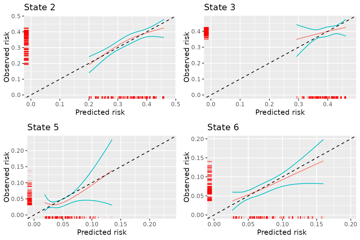
Figure 3: Calibration plots for competing risks model out of the starting state when using graphical calibration curves
Comarpsion of results
The calibration of the transition probabilities is similar irrespective of the method used to assess calibration. This is with the exception of the calibration of the transition probabilities into state 3 when using the BLR-IPCW approach. Possible reasons for this are discussed in the Evaluation-of-estimation-of-IPCWs vignette. In practice, it could be worth assessing calibration using a variety of approaches. If agreement is found, this would provide reassurance over the assessment of calibration. Note that the graphical calibration curves approach does not provide a way to assess the calibration of state 1, hence the difference in the number of plots.